1
#-- This will reseted the runtime and  clear all variable.
2
%reset -f
3
#A new Begining
4

5
#-- importing all the necessary Libraries
6
import numpy as np
7
from matplotlib import pyplot as plt
8
import ipywidgets as widgets
9
from IPython.display import display
10
## --
11

12

13
#-- Custome functions to make life easy.
14
# g3 represent Group 3
15
# g3_lable class creates a lable object which can be used with newPlot and multiPlot functions
16
# g3_lable format is
17
#1.  Legend of the plot that u want to make   )
18
#2. X axis lable ,  3. Y axis lable
19
#3 style of line ploted
20
# this can all be skiped and a defalt plot is made with defalt lable
21

22
#newPlot makes a fresh new Figure and plot taking the g3_lable
23
#formate is (x values , y values , g3_lable object )
24

25
# multiPlot can be used repeteadly to plot on same figure.
26
#formate is (x values , y values , g3_lable object ).
27

28

29
class g3_lable:      # New class to make labling easy and code smaller and reusable.
30
  def __init__(self, ll = 'not specified',lx = 'x',ly ='y',style = '-'):
31
    self.ll = ll    # the lable for legend
32
    self.lx = lx    # x axis
33
    self.ly = ly    # y axis
34
    self.style = style
35

36

37
def newPlot(x, y, L = g3_lable() ):
38

39
  fig = plt.figure()
40
  easy = fig.add_subplot(111)
41
  easy.plot( x, y,  L.style, label = L.ll )
42
  easy.legend()
43
  plt.xlabel( L.lx )
44
  plt.ylabel( L.ly )
45
  plt.show()
46

47
def multiPlot(x, y, L = g3_lable() ):
48
  plt.plot( x, y, L.style, label = L.ll ,alpha=0.5)
49
  plt.legend()
50
  plt.xlabel( L.lx )
51
  plt.ylabel( L.ly )
52
#--

Q1.#

For the radioactive decay problem discussed in class, plot the absolute difference between the numerical and analytical solutions vs time. Write down your observations from the plot - and explain the late-time characteristics.

##Solution

Theory

Nuclear decay is process where an unstable nucleus spontaneously emits energy and decays to a daughter nuclei have a lower mass.

We can find the decay equation just by thinking about it in terms of “rate of change” of N(t) is $-\frac{dN(t)}{dE}$ ,

$\Rightarrow \frac{d N}{dt} =-\lambda N(t)$

The differential equation of decay problem is $\frac{d N}{dt} = - \frac{N(t)}{\tau}$

and we get analytical solution as $N(t) = N_0 * e^{-\tau t }$

1
tau     = 5.0    # unit if time
2
N_0     = 100     # Number of Nuclei at time zero , at the begining of the system.
3
dt      = 1/100   # hundreadth of a second smallest interval of time
4
T_final  = tau *10 #  Time    # How far in time we want to do the measurment
5

6
#dont want to talk about longtime now
7
#but taking T_final 10 X longer will be more then enough for this case.
8

9
# its better to not take dt in terms of tau for abstraction.
10

11
t = np.arange(0, T_final+dt, dt)
12
N = np.zeros(len(t))
13
N[0] = N_0      # putting initial condition in the array.
14

15
# this defination is used to give value of the differential equation
16
def function(x,y):
17
  return -y /tau
18

19
# defination for solving euler equation
20
def euler( x , y ,h ):
21
  for i in range(len(x)-1):
22
    y[i+1] = y[i] + function(x[i],y[i])*h
23
  return y
24

25
#analytical solution for decay problem
26
def N_analytical(x,y_0):
27
  return (y_0 * np.exp(-x/tau))
28

29
def analytical( x , y ):
30
  for i in range(len(x)-1):
31
    y[i+1] = N_analytical(x[i+1],y[0])
32
  return y
33

34
# euler function call will creat the compleat array for number of Nuclei
35
# and store in variable N
36
N =  euler(t,N,dt)
37

38
# making plot
39
plt.figure(num=1,figsize=(10,6))
40
plt.plot (t, N, 'o', label = 'numerical')
41
plt.plot (t, N_0*np.exp(-t/tau), '-',label = 'analytic')
42
plt.legend ()
43
plt.xlabel('time')
44
plt.ylabel('Number of Nuclei')
45
plt.show()
46
# didnt write  unit(sec) in plot to variable time as it won't have any meaning.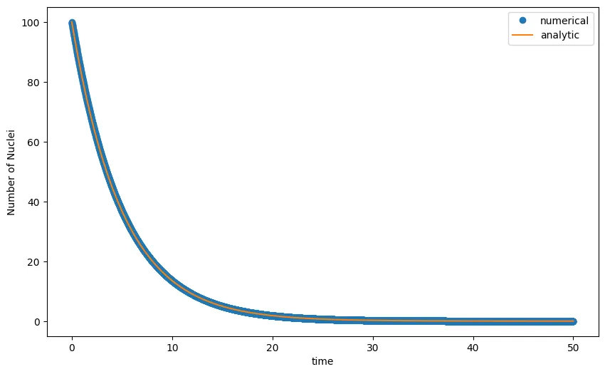

png

$\Delta N = |N_{euler} - N_{analytical} |$

$\Delta N[t] = N[t-1] - \frac{N[t-1]}{\tau} \Delta t - N[t = 0]* e^{\frac{-t}{\tau}}$

at $t= \tau , \Delta N \text{ is maximum}$

1
# finding difference in numerical and analytic
2
delta_N = np.absolute( N - N_0*np.exp(-t/tau) )
3
delta = list(delta_N)
4
print('time at max difference is t =  ',t[delta.index(max(delta))])
5

6
# using custom function to lable and plot
7
L = g3_lable('Difference','time ','difference in numerical and analytic n (t) ','--')
8
newPlot(t , delta_N, L)

1
time at max difference is t =   5.0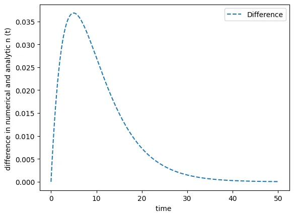

png

Following is a try at answer the question that sir asked

why the plot shifts such maximum difference is at $Time = \tau$

1
delta_N_t_euler =  -N_0*np.exp(-t/tau)/tau
2
delta_N_t_analytical = -t*N_0*np.exp(-t/tau)
3

4
delta_N = np.absolute(N - N_0*np.exp(-t/tau) )
5
del_rate = np.absolute(delta_N_t_euler - delta_N_t_analytical)
6
plt.plot (t,del_rate, label = 'rate')
7

8
plt.plot (t, delta_N, label = 'Difference')
9
delta = list(np.absolute(delta_N))
10

11
print(t[delta.index(max(delta))])
12
delta = list(np.absolute(del_rate))
13
print(t[delta.index(max(delta))])
14

15
plt.plot (t,delta_N_t_euler,'r' ,label = 'delta_N_t_euler')
16
plt.plot (t,delta_N_t_analytical,'g' ,label = 'delta_N_t_analytical')
17

18
plt.legend ()
19
plt.xlabel('t / sec')
20
plt.ylabel('difference in numerical and analytic n  (t)')
21
plt.grid(color='b', linestyle='-', linewidth=1)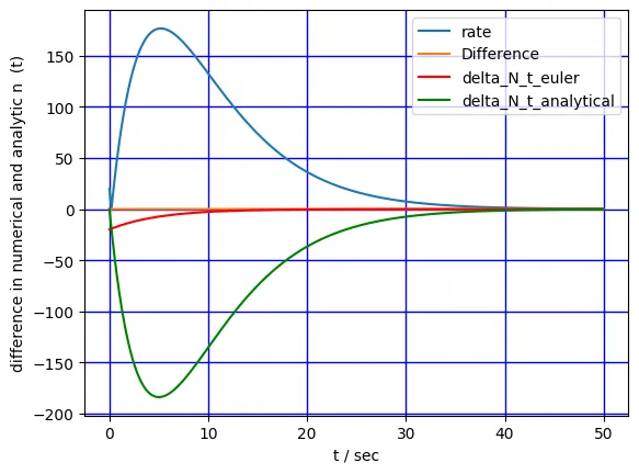
22
plt.show()

png

#Q2 The velocity of a freely falling object near the Earth’s surface is described by the equation $\frac{dv}{dt} = − g$ where $g = 9.8 m/s^2$ is the acceleration due to gravity.

Use the Euler’s method to solve this differential equation to calculate the velocity of a freely falling object in the interval $0 < t < 10 s$ , whose initial velocity at $t = 0$ is $zero$ . Repeat the calculation for different values of the time-step $\Delta t$ .
It turns out that for this case, Euler’s method gives the exact result - verify with your numerical result and prove it analytically.

Euler’s method#

In practical, many first order differential equation is difficult to, or cannot, be solved by the analytical method. In this case Euler’s method canbe used for apromimating value of first order differential equation which are difficult to solve.

We need to provided the initial condition and such problems are called initial value problem.

Assume the solution for $y=y ( x)$ exist

$y^{^{\prime }} ( x)$ can be approxiamted by $y^{^{\prime }}\left( x\right) \approx \frac{y\left( x+h\right) -y\left( x\right) }{\left( x+h\right) -x}$

And we get Euler’s method of approximation

y ( x+h) \approx y( x) +hy^{^{\prime }}( x)

##Part 1 : calculate the velocity of a freely falling object

1
velocity_0 = 0  #meter/sec initial condition.
2
time_start = 0  #sec
3
time_end   = 10 #sec
4
time_step  = 1.0 /100   #sec  Hundredth of a second
5
time       = np.arange(time_start, time_end + time_step, time_step)
6

7
print(len(time))
8

9
velocity    = np.zeros( time.size )
10
velocity[0] = velocity_0
11
print(len(velocity))
12

13
# --- set 2 conditions
14
velocity_2_0 = 0 #meter/sec initial condition.
15

16
time_step_2 = 1.0 / 50   # 50th of a sec for case 2
17
time_2      = np.arange(time_start, time_end + time_step, time_step_2)
18

19

20
velocity_2   = np.zeros( time_2.size )
21
velocity_2[0]   = velocity_2_0
22
# ---
23

24
#-- New definations to make code abstract.
25

26
def function(x,y): # dy/dx = -g.   # x y are just included for generality it does not needed.
27
  g = 9.8 #meter/sec
28
  # no need to put g here but just making sure.
29
  return -g
30

31
def euler( x , y ,h ):
32
  print(len(x-1))           # x y are arrays on whome euler method is applied with time step h
33
  for i in range( len(x) - 1 ):   # this loop goes from the index position 1 to -2
34
    y[i+1] = y[i] + function(x[i],y[i])*h #value determined for all points in time
35
  return y
36

37

38
velocity = euler( time , velocity, time_step )
39

40
lable1 = g3_lable('Eueler method dt = 1/100 sec','time sec','Velocity m/s','-r')
41
newPlot(time, velocity, lable1 )
42
#Making different plot bec they Overlap.
43
#set 2 plot
44
velocity_2 = euler( time_2 , velocity_2, time_step_2 )
45

46
lable2 = g3_lable('Eueler method dt = 1/50 sec','time sec','Velocity m/s','o')
47
newPlot(time_2, velocity_2 , lable2 )
48

49
# I am not worried about the sign convention.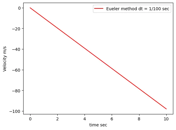

png

1
501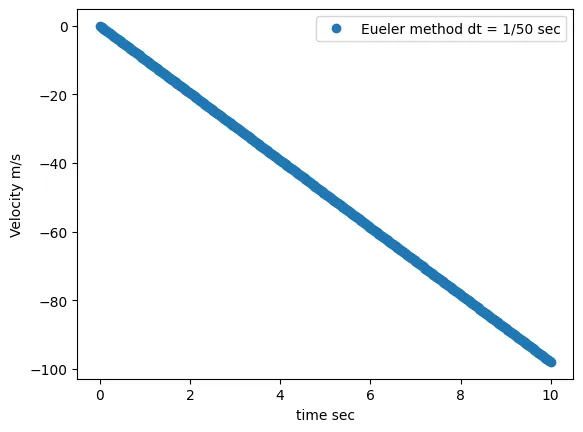

png

##Part 2 Euler vs Analytical

Proof.

Summation of $h$ over the compleat interval is the total Time leaving one element

1
velocity_0 = 0  #meter/sec initial condition.
2
time_start = 0  #sec
3
time_end   = 10 #sec
4
time_step  = 1.0 /100   #sec  Hundredth of a second
5
time       = np.arange(time_start, time_end + time_step, time_step)
6

7
velocity    = np.zeros( time.size )
8
velocity[0] = velocity_0
9

10
velocity_analytical     = np.zeros( time.size )
11
velocity_analytical [0] = velocity_0
12

13

14
def function(x,y): # dy/dx = -g.   # x y are just included for generality it does not needed.
15
  g = 9.8 #meter/sec
16
  return -g
17

18
def analytical( x , y ,y0):
19
  g = 9.8 #meter/sec
20
  y = -g * x + y0
21
  return y
22

23

24
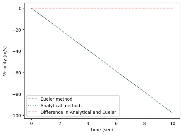
velocity     = euler( time , velocity, time_step )
25
lable1       = g3_lable('Eueler method ','time (sec)','Velocity (m/s)','--')
26
multiPlot(time, velocity, lable1 )
27

28
velocity_analytical = analytical(time , velocity_analytical, velocity_0 )
29
lable2              = g3_lable('Analytical method' ,'time sec','Velocity m/s',':k')
30
multiPlot(time, velocity_analytical, lable2 )
31

32
lable3         = g3_lable('Difference in Analytical and Eueler ','time (sec)','Velocity (m/s)','--r')
33
delta_velocity = velocity - velocity_analytical
34
multiPlot(time, delta_velocity , lable3 )
35

36
if delta_velocity.max() < pow(10,-6):
37
  print("To Notice The value of difference is very small  = {0} ".format(delta_velocity.max()))
38
  print("The Analytical and Eueler euler value overlap")
39
  # this happened bec in euler method we are using delta time and the internal rounding off by Python.
40

41
plt.plot()

1
1001
2
To Notice The value of difference is very small  = 8.100187187665142e-13
3
The Analytical and Eueler euler value overlap
4

5

6

7

8

9
[]

png

Q3#

It is often the case that frictional forces on an object increases as the object moves faster. For a parachutist, this is fortunate. The air drag allows the parachutist to land safely. Consider a simple example where the frictional force depends only on the velocity. Assume that the velocity of the object obeys an equation of the form $\frac{dv}{dt} = g − \alpha v$ , where $g = 9.8 m/s^22$ is the acceleration due to gravity and $\alpha$ is the frictional drag coefficient.

From physical considerations, what can you say about the sign of $\alpha$ ?
For the various value of $\alpha = 1, 1.5, 2.0 ,$ etc. show that a freely falling object approaches a constant velocity after long-times.
As a physicist, how would you quantify ‘long-time’ - long as compared to what? In other words, can you think of a typical time-scale in the problem?
In class, we have discussed using typical ‘scales’ in the problem to adimensionalize a given differential equation. Can you think of the different time and velocity scales in this problem and re-cast the given differential equation in dimensionless variables? Re-do the numerical solution and plot it in these new coordinates, and interpret your result.

##Part 1. Sign of $\alpha$

First lets decide the sign convention Vectores toward ground is +ve so $\vec{g} \text{ is } +ve$ (dosent matter for alpha)

$\vec{g} = +9.8 m/s$

$\alpha$ is always positive.

When an object in and fluid has any velocity irespective of it direction the drag force will alway be antiparallel to its velocity.

$\frac{d v }{dt} = g -\alpha v$

$v(t) = = \frac{g}{\alpha} + \left( v(t=0) - \frac{g}{\alpha} \right) e^ { - \alpha t}$

##Part 2. various value of $\alpha$

1
#-- initial Conditions
2
g        = 9.8   #m/s
3
alpha    = 1.0
4
alpha2   = 1.5
5
alpha3   = 2.0
6

7
velocity_0 = 0  #meter/sec initial condition.
8
#
9

10
time_start = 0  #sec
11
time_end   = 10 #sec
12
time_step  = 1.0 /100   #sec  Hundredth of a second
13
time       = np.arange(time_start, time_end + time_step, time_step)
14

15
velocity    = np.zeros( time.size )
16
velocity[0] = velocity_0
17

18
def function(t,v,alpha_i):
19
  temp = g - alpha_i * v
20
  return temp
21

22
def euler( x , y ,h ,alpha_i):
23
  for i in range(len(x)-1):
24
    y[i+1] = y[i] + function(x[i],y[i],alpha_i)*h
25
  return y
26

27
# following iss plot for cases by case basis
28

29
velocity = euler( time , velocity, time_step ,alpha)
30
lable1 = g3_lable('Eueler method alpha = {0}'.format(alpha),'time (sec)','Velocity (m/s)','--')
31
multiPlot(time, velocity, lable1 )
32
print('Terminal velocity  for  alpha = {1}  is  {0} m/s'.format( round(velocity[-1],2) ,alpha))
33

34
velocity = euler( time , velocity, time_step ,alpha2)
35
lable2 = g3_lable('Eueler method alpha = {0}'.format(alpha2),'time (sec)','Velocity (m/s)','--')
36
multiPlot(time, velocity, lable2 )
37
print('Terminal velocity  for  alpha = {1}  is  {0} m/s'.format( round(velocity[-1],2) ,alpha2))
38

39
velocity = euler( time , velocity, time_step ,alpha3)
40
lable3 = g3_lable('Eueler method alpha = {0}'.format(alpha3),'time (sec)','Velocity (m/s)','--')
41
multiPlot(time, velocity, lable3 )
42
print('Terminal velocity  for  alpha = {1}  is  {0} m/s'.format( round(velocity[-1],2) ,alpha3))
43

44
plt.show()

1
Terminal velocity  for  alpha = 1.0  is  9.8 m/s
2
Terminal velocity  for  alpha = 1.5  is  6.53 m/s
3
Terminal velocity  for  alpha = 2.0  is  4.9 m/s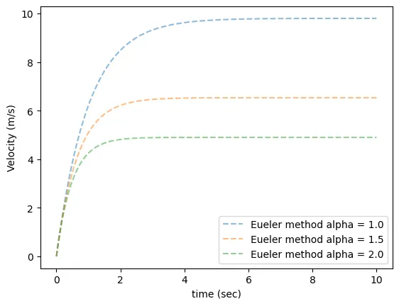

png

###Interactive

1
# This is an interactive plot for air drag equation.
2
# The interactive widgets might not work properly somtimes
3
# but reRuning same seems to resolve the  problem
4
# error is bec of the same variable is also used in other cells and being intractive its active.
5

6
# their is no need to do this initialization for velocity.
7
velocity_0 = 0  #meter/sec initial condition.
8
time_start = 0  #sec
9
time_end   = 50 #sec
10
time_step  = 1.0 /100   #sec  Hundredth of a second
11

12
g = 9.8 # m/s
13

14
time       = np.arange(time_start, time_end + time_step, time_step)
15
velocity    = np.zeros( time.size )
16
velocity[0] = velocity_0
17

18
def function(t,v,alpha_i):
19
  temp = g - alpha_i * v
20
  return temp
21

22
def euler( x , y ,h ,alpha_i):
23
  for i in range(len(x)-1):
24
    y[i+1] = y[i] + function(x[i],y[i],alpha_i)*h
25
  return y
26

27
# This function is trigered / runs when the value of the slider is changed.
28
def update_plot(alpha,velocity_Zero):
29
  velocity    = np.zeros( time.size )
30
  velocity[0] = velocity_Zero
31
  velocity = euler( time , velocity, time_step,alpha )
32
  lable1 = g3_lable('For alpha = {0} \n V(t=0) = {1} \n Terminal Velocity = {2} m/s '.format(alpha,velocity_Zero , round(velocity[-1],2) ),'time (sec)','Velocity (m/s)','--')
33
  newPlot(time, velocity, lable1 )
34
  plt.show()
35

36
#making slider for alpha , and initial velocity
37
alpha = widgets.FloatSlider(min=0, max=10, value=0,step = 0.1 , description = 'alpha : ')
38
velocity_Zero = widgets.FloatSlider(min= -50, max=50, value=0,step = 5 , description = 'Initial velocity : ')
39

40
#Starting the intractive session
41
widgets.interactive(update_plot,alpha = alpha, velocity_Zero = velocity_Zero)

1
interactive(children=(FloatSlider(value=0.0, description='alpha : ', max=10.0), FloatSlider(value=0.0, descrip…

##Part 3. Long - time.

The time scale is easy tosee in the dimensionless part.

after the dimensionless $\tau > 5$ the body has almost reached its terminal velocity and the scalling factor is $\frac{1}{\alpha}$

so the tipical time scale is like the body attends terminal velocity in $\frac{ (4 \text{ to } 6)}{ \alpha} \text{ seconds }$

Long term is indeed a subjective term,

But if we are observing a specific system we can subjectively define a long time when the variable we are observing is defined well or what follows is obvious like in the case of the freely falling body we know the speed will keep increasing (in a vacuum) under gravity, here we are only concerned about how the velocity increases or our interest is to calculate this with Euler method that is completed so we will not observe it for more than 10-sec eas we know that velocity will keep increasing until it hits earth surface, but see we don’t need to keep measuring velocity until it hits surface because we are not interested in that part.

Following might be wrong . “I will stop doing observation if the values, In last 10 percent of the time (wrt total time observed) had just increased 1 percent( wrt total change). Or something like to compare the rate of change (of what we interested) with log base e. , is this long time ? No , That what I would say if i am bored I won’t do more observation ”

by one of our team member .

##Part 4. Non Dimensionalization.

To Make $\frac{dv}{dt}=g - \alpha v$ dimensionless

Variables: $v$ , $t$ parameter: $g$ , $\alpha$

Let $u = \frac{v}{W_0}$ and $\tau = t / T_0$

substituting this value in $\frac{dv}{dt}=g - \alpha v$

as $v = u W_0$ $t = \tau T_0$

$\frac{d uW_0}{d\tau T_0} = g - \alpha u W_0$

$\frac{d u}{d\tau } = \frac{T_0 g}{W+0} - T_0 \alpha u W_0$

Let $T_0 \alpha = 1$

$\Rightarrow T_0 = \frac{1}{\alpha}$

Let $\frac{T_0}{W_0} g = 1$

$W_0 = T_0 h$

$\Rightarrow W_0 = \frac{g}{\alpha}$

So the New Differential Equation is $\frac{du}{d \tau} = 1- u$

scalling factors $v = \frac{g}{\alpha} u , t = \frac{1}{\alpha} \tau$

1
g        = 9.8 # m/s
2
alpha    = 2.0
3

4
T_not  =  1/alpha # t0 = 1/alpha This is scalling factor for time
5
W_not  =  g/alpha # Scalling factor for velocity
6

7
#T his is non dim variable U_velocity and Tau_t
8
U_velocity_0 = 0
9
Tau_t_start = 0
10
Tau_t_final   = 10
11
Tau_t_step  = 1.0 /100   #sec  Hundredth of a second
12
Tau_t       = np.arange(Tau_t_start, Tau_t_final + Tau_t_step, Tau_t_step)
13

14
U_velocity    = np.zeros( Tau_t.size )
15
U_velocity[0] = U_velocity_0
16

17
def function(v):
18
  #temp = 1 - 1 * v
19
  return 1 - 1 * v
20

21
def euler( x , y ,h ):
22
  for i in range(len(x)-1):
23
    y[i+1] = y[i] + function(y[i])*h
24
  return y
25

26
U_velocity = euler( Tau_t , U_velocity, Tau_t_step)
27

28
lable1 = g3_lable('Euler method with Non dimension ','Tau_t','U_velocity ','--')
29
multiPlot(Tau_t, U_velocity, lable1 )
30

31

32
lable2 = g3_lable('Eueler method with Non dimension ','time (sec)','velocity (m/s)','--')
33
# plot with scalling factors
34
newPlot(Tau_t * T_not , U_velocity * W_not, lable2 )
35

36
print('Terminal velocity  for  alpha = {1}  is  {0} m/s'.format( round(U_velocity[-1] * W_not,2) ,alpha))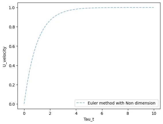

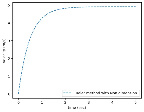
png

1
Terminal velocity  for  alpha = 2.0  is  4.9 m/s

#Q4 Consider a radioactive decay problem involving two types of radioactive nuclei - A and B with populations $N_A (t)$ and $N_B (t)$ . Suppose type A nuclei decay to form type B nuclei, which then also decay according to the differential equations.

$\frac{d N_A(t)}{dt} = -\frac{N_A(t)}{\tau}$

$\frac{d N_B(t)}{dt} = \frac{N_A(t)}{\tau_A} -\frac{N_B(t)}{\tau_B}$

where $\tau_A$ & $\tau_B$ and are the decay time constants for each type of nucleus.

Use the Euler method to solve these coupled equations for $N_A(t)$ and $N_B(t)$
Obtain an analytic solution for $N (t)$ and and compare them with your numerical result.
It is interesting to explore the behaviour found for different values of the ratio $\frac{\tau_A}{\tau_B}$ . In particular, try to interpret the short and long time behaviour for different values of this ratio.

##Part 1. Coupled Equations. $\frac{d N_A(t)}{dt} = -\frac{N_A(t)}{\tau}$

$\frac{d N_B(t)}{dt} = \frac{N_A(t)}{\tau_A} -\frac{N_B(t)}{\tau_B}$

1
#Defining the initial conditions.
2

3
N_A0,   N_B0      = 100,  0
4
tauA,   tauB      = 1  ,  3
5

6
t0, T_final = 0, 10
7
dt         = 0.01
8

9
#--
10
# Defining the variables.
11
time  = np.arange(t0, T_final+dt, dt)
12

13
N_A = np.zeros(time.size)
14
N_B = np.zeros(time.size)
15
N_A[0], N_B[0] = N_A0 , N_B0
16

17
#ODE for parent nuclei
18
def ode_A(y):
19
  return -y /tauA
20

21
#ODE for daughter nuclei
22
def ode_B(y,y2):
23
  return y /tauA - y2 /tauB
24

25
def euler( x , y , y2 ,h ):
26
  for i in range(len(x)-1):
27
    y[i+1] = y[i] + ode_A( y[i] )*h
28
    y2[i+1] = y2[i] + ode_B(y[i], y2[i] )*h
29
  return y,y2
30

31
#Getting numbers of both nuclei by solving ode
32
N_A, N_B = euler(time, N_A, N_B ,dt )
33

34
# following is Plot
35

36
lable1 = g3_lable('Tau = {0}'.format(tauA),'time (sec)','Number of nuclei','b+')
37
multiPlot(time, N_A, lable1 )
38

39
lable2 = g3_lable(' Tau = {0}'.format(tauB),'time (sec)','Number of nuclei ','or')
40
multiPlot(time, N_B, lable2 )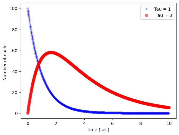
41
plt.plot()

1
[]

png

##Part 2. analytic solution for $𝑁(𝑡)$

1
# the Code currently suports the Daughter nuclie initial population zero.
2
#N_B0 =0 compulsory only for analytical solution.
3

4
N_A0,   N_B0      = 100,  0
5
tauA,   tauB      = 1  ,  3
6

7
t0, T_final = 0, 10
8
dt         = 0.1
9

10
#--
11
# Defining the variables.
12
time  = np.arange(t0, T_final+dt, dt)
13

14
N_A = np.zeros(time.size)
15
N_B = np.zeros(time.size)
16
N_A[0], N_B[0] = N_A0 , N_B0
17

18
N_A_analytical = np.zeros(time.size)
19
N_B_analytical = np.zeros(time.size)
20
N_A_analytical[0] = N_A0
21
N_B_analytical[0] = N_B0
22

23

24
#ODE for parent nuclei
25
def ode_A(y):
26
  return -y /tauA
27

28
#ODE for daughter nuclei
29
def ode_B(y,y2):
30
  return y /tauA - y2 /tauB
31

32
#analytical solution N_A
33
def NA_analytical(x,y_0):
34
  return (y_0 * np.exp(-x/tauA))
35

36
#analytical solution N_B
37
def NB_analytical(x,y_0):
38
  temp = tauB/(tauA - tauB) * y_0*(np.exp(-x/tauA)-np.exp(-x/tauB))
39
  return temp
40

41
# this function is not implimented as this needs to be corrected.
42
def NB_non0_analytical(t,y1_0,y2_0):
43

44
  temp = tauA * y2_0 * np.exp(-t/tauB)
45
  temp = temp + tauB*( y1_0 * np.exp(-t/tauA ) - np.exp(-t / tauB) )
46
  temp = temp / (tauA-tauB )
47

48
  return temp
49

50
def euler( x , y , y2 ,h ):
51
  for i in range(len(x)-1):
52
    y[i+1] = y[i] + ode_A( y[i] )*h
53
    y2[i+1] = y2[i] + ode_B(y[i], y2[i] )*h
54
  return y,y2
55

56
#Getting numbers of both nuclei by solving ode
57
N_A, N_B = euler(time, N_A, N_B ,dt )
58

59
N_A_analytical = NA_analytical(time,N_A0)
60
N_B_analytical = NB_analytical(time, N_A0 )
61
#N_B_analytical = NB_non0_analytical(time , N_A0 , N_B0)
62

63
# following is Plot for euler
64
lable1 = g3_lable('Tau = {0}'.format(tauA),'time (sec)','Number of nuclei','b+')
65
multiPlot(time, N_A, lable1 )
66

67
lable2 = g3_lable(' Tau = {0}'.format(tauB),'time (sec)','Number of nuclei ','or')
68
multiPlot(time, N_B, lable2 )
69

70
plt.title("Solution by Euler method")
71
#this will end the current instanceof multiplot.
72
plt.show()
73

74
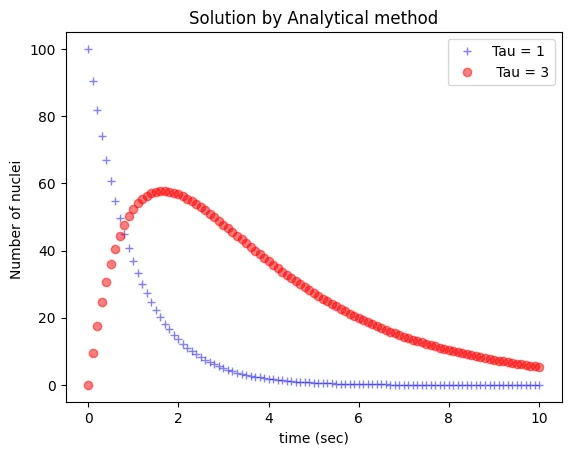
# following is Plot for numerical
75
lable1 = g3_lable('Tau = {0}'.format(tauA),'time (sec)','Number of nuclei','b+')
76
multiPlot(time, N_A_analytical, lable1 )
77

78
lable2 = g3_lable(' Tau = {0}'.format(tauB),'time (sec)','Number of nuclei ','or')
79
multiPlot(time, N_B_analytical, lable2 )
80
plt.title("Solution by Analytical method")
81
plt.show()
82

83
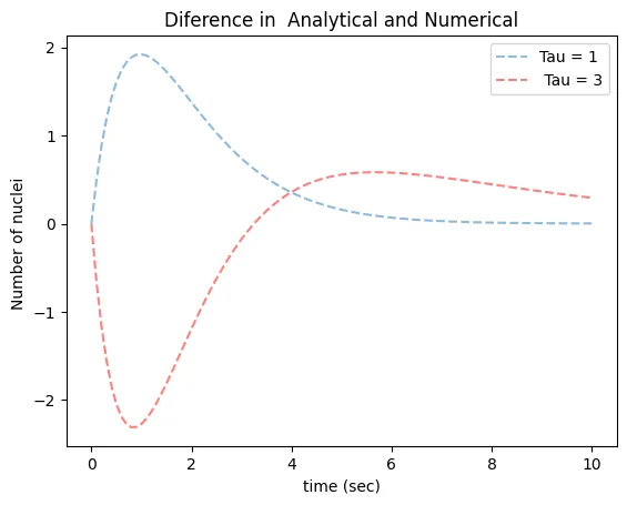
Difference_N_A = N_A_analytical - N_A
84
Difference_N_B = N_B_analytical - N_B
85

86
lable1 = g3_lable('Tau = {0}'.format(tauA),'time (sec)','Number of nuclei','--')
87
multiPlot(time, Difference_N_A, lable1 )
88
plt.title("Diference in  Analytical and Numerical")
89

90
lable2 = g3_lable(' Tau = {0}'.format(tauB),'time (sec)','Number of nuclei ','--r')
91
multiPlot(time, Difference_N_B, lable2 )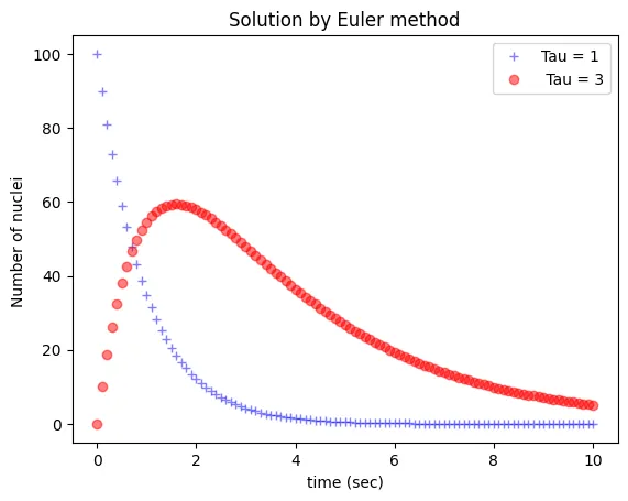

png

##Part 3. behaviour found for different values of the ratio

1
N_A0,   N_B0  = 100,  0
2
t0, T_final    = 0, 10
3

4
dt = 0.1
5
#
6

7
tauA,tauB     = 1  ,  3
8

9
#--
10
# Defining the variables.
11
time  = np.arange(t0, T_final+dt, dt)
12

13
N_A = np.zeros(time.size)
14
N_B = np.zeros(time.size)
15
N_A[0], N_B[0] = N_A0 , N_B0
16

17
#definations made for interactive plot.
18

19
def eulerI( x , y , y2 ,h ):
20
  for i in range(len(x)-1):
21
    y[i+1] = y[i] + ode_AI( y[i] )*h
22
    y2[i+1] = y2[i] + ode_BI(y[i], y2[i] )*h
23
  return y,y2
24

25
def ode_AI(y):
26
  return -y /tauA_interactive.value
27

28
#ODE for daughter nuclei
29
def ode_BI(y,y2):
30
  return y /tauA_interactive.value - y2 /tauB_interactive.value
31

32

33
def update_plot(tauA,tauB,NB_initial):
34
  N_A = np.zeros(time.size)
35
  N_B = np.zeros(time.size)
36
  N_A[0], N_B[0] = N_A0 , NB_initial
37
  N_A, N_B = eulerI(time, N_A, N_B ,dt )
38

39
  lable1 = g3_lable('Tau A = {0}'.format(tauA),'time (sec)','Number of nuclei','b+')
40
  multiPlot(time, N_A, lable1 )
41

42
  lable2 = g3_lable(' Tau B = {0}'.format(tauB),'time (sec)','Number of nuclei ','or')
43
  multiPlot(time, N_B, lable2 )
44
  plt.title(' Solution by Euler methot for tauA / tauB  = {0}'.format(tauA/tauB))
45
  plt.show()
46

47
#making slider for alpha , and initial velocity
48
tauA_interactive = widgets.FloatSlider(min=0, max=10, value=1,step = 0.5 , description = 'Tau A : ')
49
tauB_interactive = widgets.FloatSlider(min= 0, max=10, value=3,step = 0.5 , description = 'Tau B  : ')
50

51
NB_interactive = widgets.FloatSlider(min= 0, max=100, value=0 ,step = 5  , description = 'Initial N B   : ')
52

53

54
#Starting the intractive session
55
widgets.interactive(update_plot,tauA = tauA_interactive, tauB =tauB_interactive,NB_initial = NB_interactive)

1
interactive(children=(FloatSlider(value=1.0, description='Tau A : ', max=10.0, step=0.5), FloatSlider(value=3.…

The End Open Lab 2#

https://github.com/ashwin-r-k/Computational-Physics_3labs/blob/main/LAB_2.ipynb