

Literature Review on Analysis of the Foucault Pendulum by D’Alembert Principle and Numerical Simulation
📚 Main Source
Title: Analysis on the Foucault Pendulum by D’Alembert Principle and Numerical Simulation
Link: arXiv:1504.03873
Publication Year: 2015
🌐 Related Resources
📝 Introduction
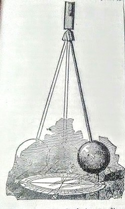
The Foucault pendulum, developed by Léon Foucault, was an experimental demonstration of the rotation of Earth. Extensively studied in the 1850s, it provided convincing experimental proof even before complete mathematical formalism was established. It also played a role in making physics accessible to the general public.
The first such pendulum used:
- A 28 kg brass-coated lead bob
- A 67-meter long wire
- Conducted at Paris Observatory, showing a full rotation period of ~31.8 hours
Behavior by Latitude:
- Poles: The plane of oscillation remains fixed; Earth rotates beneath it.
- Viewed from above:
- North Pole → clockwise rotation in 24 hrs
- South Pole → counterclockwise
- Viewed from above:
- Equator: No apparent precession
- Other latitudes: Plane precesses more slowly; full rotation takes more than 24 hrs
📖 Description
The Foucault pendulum exhibits precessional motion due to the Earth’s rotation and the pendulum’s oscillation. Accurately solving for its motion is complex as it must include:
- Gravity
- Tension
- Coriolis force
Earlier models assumed small amplitude oscillations, simplifying the equations (e.g., Eq. O.1, O.2). However, this study:
- Focuses on both small and large amplitude cases
- Uses D’Alembert’s Principle for theoretical modeling
- Applies Runge-Kutta method for numerical analysis
Modeling Assumptions:
-
Massless string
-
Point mass bob
-
Uniform gravitational field
-
Earth approximated as a sphere
-
No variation in latitude-longitude gravitational effects
-
Fig. 2: Chosen coordinate system
-
Tension forces avoided using D’Alembert’s Principle
Simulation:
- Runge-Kutta method chosen for high-accuracy numerical results
- Fig. 3 to 8: Pendulum’s projected motion on the horizontal plane
- Graphs plotted as:
- y/l vs x/l to visualize motion trails
- z/l vs t to show vertical oscillation behavior
From Fig. 9 and 10, it is evident that:
- The vertical motion is simple harmonic
- Its projection behaves as oscillation in z-direction
✅ Conclusion
The study examines both small and large amplitude scenarios, comparing theoretical and numerical models.
- For small amplitudes: Minimal difference between theory and simulation
- For large amplitudes: Clear deviation appears, highlighting non-linear effects
The Foucault pendulum problem is modeled effectively using:
- D’Alembert Principle
- Runge-Kutta numerical simulations
These analyses offer clear insight into the complex and elegant behavior of the Foucault pendulum system.